Note
Click here to download the full example code
Quick start
The examplar data to replicate the figure in the jupyter notebook can be found here.
The data contains a sample recordings taken simultaneously from the anterodorsal thalamus and the hippocampus and contains both a sleep and wake session. It contains both head-direction cells (i.e. cells that fire for a particular head direction in the horizontal plane) and place cells (i.e. cells that fire for a particular position in the environment).
Preprocessing of the data was made with Kilosort 2.0 and spike sorting was made with Klusters.
Instructions for installing pynapple can be found here.
This notebook is meant to provide an overview of pynapple by going through:
- Input output (IO). In this case, pynapple will load a NWB file using the NWBFile object within a project Folder that represent a dataset.
- Core functions that handle time series, interval sets and groups of time series. See this notebook for a detailled usage of the core functions.
- Process functions. A small collection of high-level functions widely used in system neuroscience. This notebook details those functions.
Warning
This tutorial uses seaborn and matplotlib for displaying the figure.
You can install both with pip install matplotlib seaborn
import numpy as np
import pandas as pd
import pynapple as nap
import matplotlib.pyplot as plt
import seaborn as sns

custom_params = {"axes.spines.right": False, "axes.spines.top": False}
sns.set_theme(style="ticks", palette="colorblind", font_scale=1.5, rc=custom_params)
IO
The first step is to give the path to the data folder.
We can load the session with the function load_folder. Pynapple will walks throught the folder and collects every subfolders.
We can use the attribute view or the function expand to display a tree view of the dataset. The treeview shows all the compatible data format (i.e npz files or NWBs files) and their equivalent pynapple type.
Out:
📂 MyProject
└── 📂 sub-A2929
    └── 📂 ses-A2929-200711
        ├── 📂 derivatives
        │   ├── spikes.npz      |        TsGroup
        │   ├── sleep_ep.npz    |        IntervalSet
        │   ├── position.npz    |        TsdFrame
        │   └── wake_ep.npz     |        IntervalSet
        ├── 📂 pynapplenwb
        │   ├── A2929-200711_nc         |        NWB file
        │   └── A2929-200711    |        NWB file
        ├── x_plus_1.npz    |        Tsd
        ├── x_plus_y.npz    |        Tsd
        └── stimulus-fish.npz       |        IntervalSet
The object data is a Folder object that allows easy navigation and interaction with a dataset.
In this case, we want to load the NWB file in the folder /pynapplenwb. Data are always lazy loaded. No time series is loaded until it's actually called.
When calling the NWB file, the object nwb is an interface to the NWB file. All the data inside the NWB file that are compatible with one of the pynapple objects are shown with their corresponding keys.
Out:
A2929-200711
┍━━━━━━━━━━━━━━━━━━━━━━━┯━━━━━━━━━━━━━┑
│ Keys                  │ Type        │
┝━━━━━━━━━━━━━━━━━━━━━━━┿━━━━━━━━━━━━━┥
│ units                 │ TsGroup     │
│ position_time_support │ IntervalSet │
│ epochs                │ IntervalSet │
│ z                     │ Tsd         │
│ y                     │ Tsd         │
│ x                     │ Tsd         │
│ rz                    │ Tsd         │
│ ry                    │ Tsd         │
│ rx                    │ Tsd         │
┕━━━━━━━━━━━━━━━━━━━━━━━┷━━━━━━━━━━━━━┙
We can individually call each object and they are actually loaded.
units is a TsGroup object. It allows to group together time series with different timestamps and couple metainformation to each neuron. In this case, the location of where the neuron was recorded has been added when loading the session for the first time.
We load units as spikes
Out:
  Index      rate  location      group
-------  --------  ----------  -------
      0   7.30358  adn               0
      1   5.73269  adn               0
      2   8.11944  adn               0
      3   6.67856  adn               0
      4  10.7712   adn               0
      5  11.0045   adn               0
      6  16.5164   adn               0
      7   2.19674  ca1               1
      8   2.0159   ca1               1
      9   1.06837  ca1               1
     10   3.91847  ca1               1
     11   3.30844  ca1               1
     12   1.0942   ca1               1
     13   1.27921  ca1               1
     14   1.32338  ca1               1
In this case, the TsGroup holds 15 neurons and it is possible to access, similar to a dictionnary, the spike times of a single neuron:
Out:
Time (s)
0.00845
0.03265
0.1323
0.3034
0.329
0.661
0.671
0.70995
1.5596
1.83285
1.8503
1.8595
1.88455
1.9147
1.9598
2.03655
2.088
2.108
2.12555
2.4989
2.5247
2.55135
3.98705
4.35335
4.6474
4.65685
4.6622
4.6698
4.68835
4.74365
...
1185.13315
1185.1391
1185.15235
1185.15935
1185.16715
1185.1747
1185.18855
1185.2097
1185.21395
1185.23365
1185.266
1185.27545
1185.28575
1185.29245
1185.30375
1185.31475
1185.3214
1185.33505
1185.34715
1185.3705
1185.3779
1185.3826
1185.39065
1185.4003
1185.84315
1186.12755
1189.384
1194.13475
1196.2075
1196.67675
shape: 8764
neuron_0 is a Ts object containing the times of the spikes.
The other information about the session is contained in nwb["epochs"]. In this case, the start and end of the sleep and wake epochs. If the NWB time intervals contains tags of the epochs, pynapple will try to group them together and return a dictionnary of IntervalSet instead of IntervalSet.
Out:
{'sleep':       start    end
 0        0    600
shape: (1, 2), time unit: sec., 'wake':       start    end
 0      600   1200
shape: (1, 2), time unit: sec.}
Finally this dataset contains tracking of the animal in the environment. rx, ry, rz represent respectively the roll, the yaw and the pitch of the head of the animal. x and z represent the position of the animal in the horizontal plane while y represents the elevation.
Here we load only the head-direction as a Tsd object.
Out:
Time (s)
----------  -------
670.6407    5.20715
670.649     5.18103
670.65735   5.15551
670.66565   5.13654
670.674     5.12085
670.68235   5.10845
670.69065   5.09732
670.699     5.08613
670.70735   5.07296
670.71565   5.06046
670.724     5.04562
670.73235   5.02894
670.74065   5.00941
670.749     4.9876
670.75735   4.96359
670.76565   4.94159
670.774     4.92152
670.78235   4.90635
670.79065   4.89627
670.799     4.89221
670.80735   4.89392
670.81565   4.89657
670.824     4.89862
670.83235   4.89802
670.84065   4.89324
670.849     4.88399
670.85735   4.86988
670.86565   4.85158
670.874     4.837
670.88235   4.82126
...
1199.7533   4.59287
1199.7616   4.57209
1199.76995  4.549
1199.77825  4.52208
1199.7866   4.49335
1199.79495  4.45941
1199.80325  4.42248
1199.8116   4.39031
1199.81995  4.35454
1199.82825  4.3253
1199.8366   4.29808
1199.84495  4.2702
1199.85325  4.24382
1199.8616   4.20729
1199.86995  4.16671
1199.87825  4.12178
1199.8866   4.07674
1199.89495  4.02607
1199.90325  3.97859
1199.9116   3.92706
1199.91995  3.87269
1199.92825  3.82848
1199.9366   3.78868
1199.94495  3.74765
1199.95325  3.70803
1199.9616   3.66595
1199.96995  3.63462
1199.97825  3.61785
1199.9866   3.60945
1199.99495  3.60938
dtype: float64, shape: (63527,)
Core
The core functions of pynapple provides many ways to manipulate time series. In this example, spike times are restricted to the wake epoch. Notice how the frequencies change from the original object.
Out:
  Index      rate  location      group
-------  --------  ----------  -------
      0   4.84667  adn               0
      1   8.06333  adn               0
      2   7.10667  adn               0
      3   7.66333  adn               0
      4   7.96833  adn               0
      5  11.285    adn               0
      6  22.0833   adn               0
      7   1.82     ca1               1
      8   2.83667  ca1               1
      9   0.705    ca1               1
     10   4.775    ca1               1
     11   4.93     ca1               1
     12   1.71     ca1               1
     13   0.96833  ca1               1
     14   0.26167  ca1               1
The same operation can be applied to all time series.
# In this example, we want all the epochs for which position in `x` is above a certain threhsold. For this we use the function `threshold`.
posx = nwb["x"]

threshold = 0.08

posxpositive = posx.threshold(threshold)

plt.figure()
plt.plot(posx)
plt.plot(posxpositive, ".")
plt.axhline(threshold)
plt.xlabel("Time (s)")
plt.ylabel("x")
plt.title("x > {}".format(threshold))
plt.tight_layout()
plt.show()
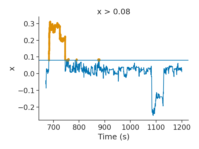
The epochs above the threshold can be accessed through the time support of the Tsd object. The time support is an important concept in the pynapple package. It helps the user to define the epochs for which the time serie should be defined. By default, Ts, Tsd and TsGroup objects possess a time support (defined as an IntervalSet). It is recommended to pass the time support when instantiating one of those objects.
Out:
      start      end
 0  682.661  745.566
 1  752.24   752.44
 2  752.582  752.674
 3  757.498  758.998
 4  789.863  790.272
 5  875.225  876.067
 6  878.158  878.642
shape: (7, 2), time unit: sec.
Tuning curves
Let's do a more advanced analysis. Neurons from ADn (group 0 in the spikes group object) are know to fire for a particular direction. Therefore, we can compute their tuning curves, i.e. their firing rates as a function of the head-direction of the animal in the horizontal plane (ry). To do this, we can use the function compute_1d_tuning_curves. In this case, the tuning curves are computed over 120 bins and between 0 and 2$\pi$.
tuning_curves = nap.compute_1d_tuning_curves(
    group=spikes, feature=head_direction, nb_bins=121, minmax=(0, 2 * np.pi)
)

print(tuning_curves)
Out:
                 0    1         2   ...         12        13        14
0.025964  45.520459  0.0  0.000000  ...  14.483782  0.000000  2.069112
0.077891  55.049762  0.0  0.000000  ...   1.100995  0.000000  0.000000
0.129818  76.369034  0.0  0.000000  ...   9.351310  1.558552  0.000000
0.181745  82.179721  0.0  0.000000  ...   9.131080  2.608880  0.000000
0.233672  73.851374  0.0  0.000000  ...   7.912647  2.637549  0.000000
...             ...  ...       ...  ...        ...       ...       ...
6.049513  15.001060  0.0  0.000000  ...   0.000000  0.000000  1.363733
6.101440  22.327159  0.0  0.000000  ...   2.790895  0.000000  0.000000
6.153367  47.062150  0.0  0.000000  ...   0.000000  2.353107  0.000000
6.205295  56.003958  0.0  2.000141  ...   6.000424  0.000000  0.000000
6.257222  38.712414  0.0  0.000000  ...   7.742483  0.000000  0.000000

[121 rows x 15 columns]
We can plot tuning curves in polar plots.
neuron_location = spikes.get_info("location")  # to know where the neuron was recorded
plt.figure(figsize=(12, 9))

for i, n in enumerate(tuning_curves.columns):
    plt.subplot(3, 5, i + 1, projection="polar")
    plt.plot(tuning_curves[n])
    plt.title(neuron_location[n] + "-" + str(n), fontsize=18)

plt.tight_layout()
plt.show()
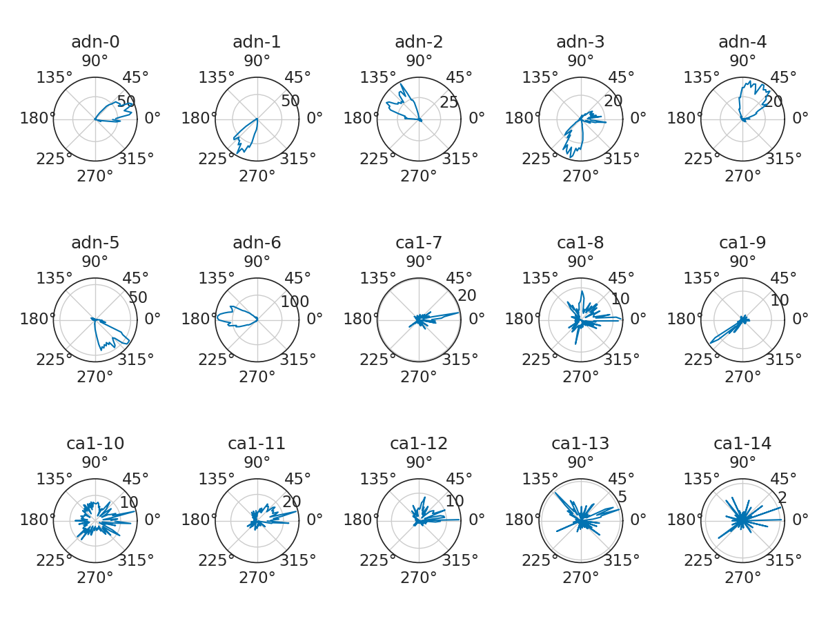
While ADN neurons show obvious modulation for head-direction, it is not obvious for all CA1 cells. Therefore we want to restrict the remaining of the analyses to only ADN neurons. We can split the spikes group with the function getby_category.
spikes_by_location = spikes.getby_category("location")

print(spikes_by_location["adn"])
print(spikes_by_location["ca1"])

spikes_adn = spikes_by_location["adn"]
Out:
  Index      rate  location      group
-------  --------  ----------  -------
      0   7.30358  adn               0
      1   5.73269  adn               0
      2   8.11944  adn               0
      3   6.67856  adn               0
      4  10.7712   adn               0
      5  11.0045   adn               0
      6  16.5164   adn               0
  Index     rate  location      group
-------  -------  ----------  -------
      7  2.19674  ca1               1
      8  2.0159   ca1               1
      9  1.06837  ca1               1
     10  3.91847  ca1               1
     11  3.30844  ca1               1
     12  1.0942   ca1               1
     13  1.27921  ca1               1
     14  1.32338  ca1               1
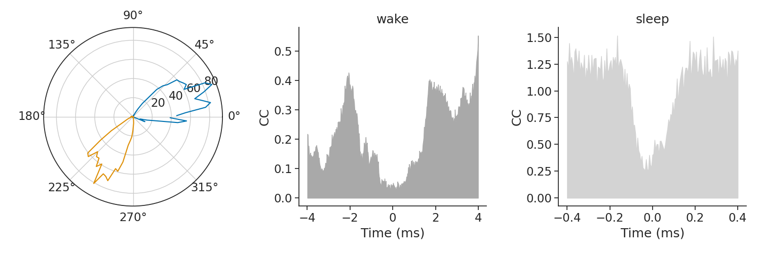
Correlograms
A classical question with head-direction cells is how pairs stay coordinated across brain states i.e. wake vs sleep (see Peyrache, A., Lacroix, M. M., Petersen, P. C., & Buzsáki, G. (2015). Internally organized mechanisms of the head direction sense. Nature neuroscience, 18(4), 569-575.)
In this example, this coordination across brain states will be evaluated with cross-correlograms of pairs of neurons. We can call the function compute_crosscorrelogram during both sleep and wake epochs.
cc_wake = nap.compute_crosscorrelogram(
    group=spikes_adn,
    binsize=20,  # ms
    windowsize=4000,  # ms
    ep=epochs["wake"],
    norm=True,
    time_units="ms",
)

cc_sleep = nap.compute_crosscorrelogram(
    group=spikes_adn,
    binsize=5,  # ms
    windowsize=400,  # ms
    ep=epochs["sleep"],
    norm=True,
    time_units="ms",
)
From the previous figure, we can see that neurons 0 and 1 fires for opposite directions during wake. Therefore we expect their cross-correlograms to show a trough around 0 time lag, meaning those two neurons do not fire spikes together. A similar trough during sleep for the same pair thus indicates a persistence of their coordination even if the animal is not moving its head. mkdocs_gallery_thumbnail_number = 3
xtwake = cc_wake.index.values
xtsleep = cc_sleep.index.values

plt.figure(figsize=(15, 5))
plt.subplot(131, projection="polar")
plt.plot(tuning_curves[[0, 1]])  # The tuning curves of the pair [0,1]
plt.subplot(132)
plt.fill_between(
    xtwake, np.zeros_like(xtwake), cc_wake[(0, 1)].values, color="darkgray"
)
plt.title("wake")
plt.xlabel("Time (ms)")
plt.ylabel("CC")
plt.subplot(133)
plt.fill_between(
    xtsleep, np.zeros_like(xtsleep), cc_sleep[(0, 1)].values, color="lightgrey"
)
plt.title("sleep")
plt.xlabel("Time (ms)")
plt.ylabel("CC")
plt.tight_layout()
plt.show()
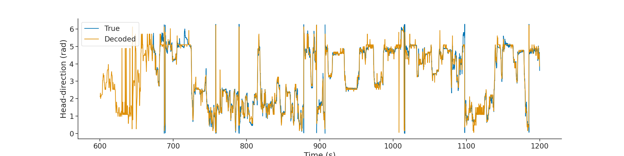
Decoding
This last analysis shows how to use the pynapple's decoding function.
The previous result indicates a persistent coordination of head-direction cells during sleep. Therefore it is possible to decode a virtual head-direction signal even if the animal is not moving its head.
This example uses the function decode_1d which implements bayesian decoding (see : Zhang, K., Ginzburg, I., McNaughton, B. L., & Sejnowski, T. J. (1998). Interpreting neuronal population activity by reconstruction: unified framework with application to hippocampal place cells. Journal of neurophysiology, 79(2), 1017-1044.)
First we can validate the decoding function with the real position of the head of the animal during wake.
tuning_curves_adn = nap.compute_1d_tuning_curves(
    spikes_adn, head_direction, nb_bins=61, minmax=(0, 2 * np.pi)
)

decoded, proba_angle = nap.decode_1d(
    tuning_curves=tuning_curves_adn,
    group=spikes_adn,
    ep=epochs["wake"],
    bin_size=0.3,  # second
    feature=head_direction,
)
print(decoded)
Out:
Time (s)
----------  -------
600.15      2.11156
600.45      2.11156
600.75      2.31757
601.05      2.00856
601.35      2.11156
601.65      2.11156
601.95      2.21457
602.25      2.21457
602.55      2.21457
602.85      2.21457
603.15      2.21457
603.45      2.42057
603.75      3.03859
604.05      3.03859
604.35      3.2446
604.65      3.4506
604.95      3.2446
605.25      3.2446
605.55      3.3476
605.85      2.93559
606.15      2.93559
606.45      2.72958
606.75      2.62658
607.05      2.52357
607.35      2.62658
607.65      2.52357
607.95      2.52357
608.25      2.83258
608.55      2.93559
608.85      2.93559
...
1191.15     4.78964
1191.45     4.78964
1191.75     4.78964
1192.05     4.89264
1192.35     5.09865
1192.65     4.89264
1192.95     4.99565
1193.25     4.99565
1193.55     4.89264
1193.85     4.78964
1194.15     4.89264
1194.45     4.78964
1194.75     4.48063
1195.05     4.48063
1195.35     4.48063
1195.65     4.99565
1195.95     4.99565
1196.25     4.89264
1196.55     4.89264
1196.85     4.78964
1197.15     4.48063
1197.45     4.27463
1197.75     4.27463
1198.05     4.58364
1198.35     4.99565
1198.65     4.58364
1198.95     4.27463
1199.25     4.58364
1199.55     4.58364
1199.85     3.86261
dtype: float64, shape: (2000,)
We can plot the decoded head-direction along with the true head-direction.
plt.figure(figsize=(20, 5))
plt.plot(head_direction.as_units("s"), label="True")
plt.plot(decoded.as_units("s"), label="Decoded")
plt.legend()
plt.xlabel("Time (s)")
plt.ylabel("Head-direction (rad)")
plt.show()
Raster
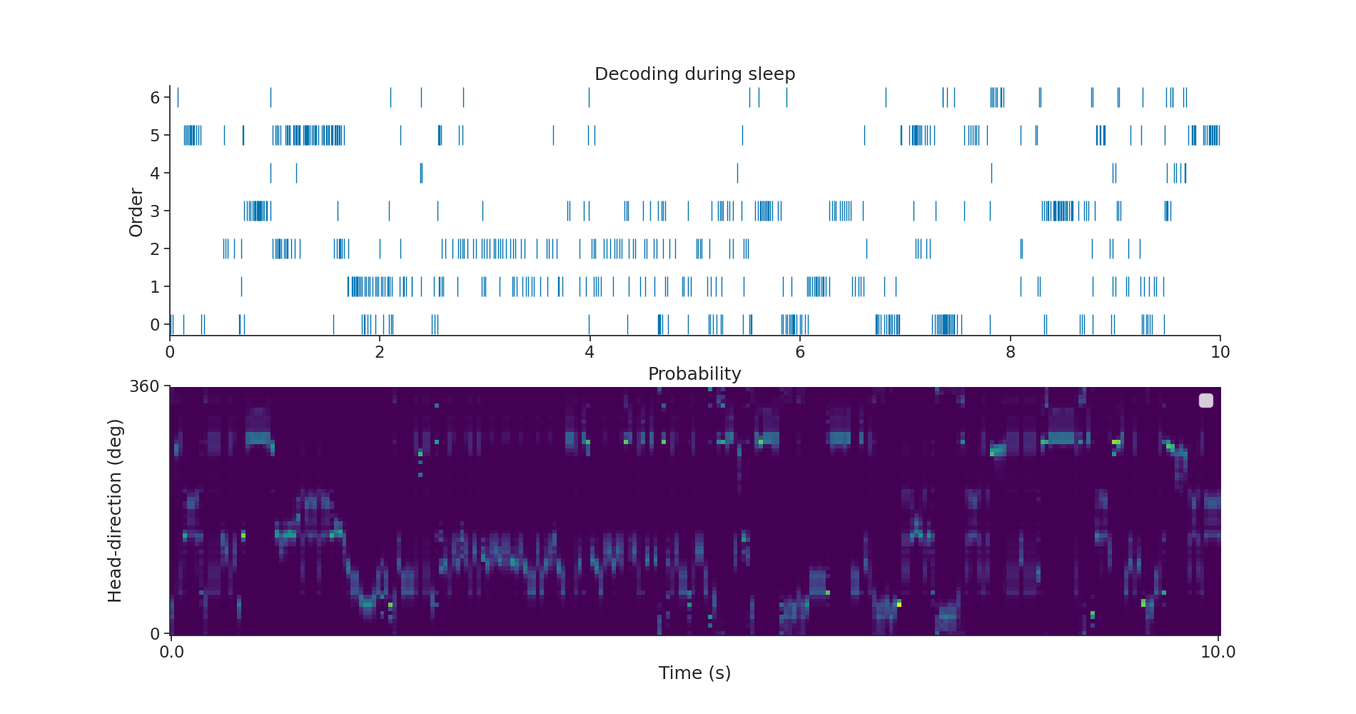
Finally we can decode activity during sleep and overlay spiking activity of ADN neurons as a raster plot (in this case only during the first 4 seconds). Pynapple return as well the probability of being in a particular state. We can display it next to the spike train.
First let's decode during sleep with a bin size of 40 ms.
decoded_sleep, proba_angle_Sleep = nap.decode_1d(
    tuning_curves=tuning_curves_adn,
    group=spikes_adn,
    ep=epochs["sleep"],
    bin_size=0.04,  # second
    feature=head_direction,
)
Here we are gonna chain the TsGroup function set_info and the function to_tsd to flatten the TsGroup and quickly assign to each spikes a corresponding value found in the metadata table. Any columns of the metadata table can be assigned to timestamps in a TsGroup.
Here the value assign to the spikes comes from the preferred firing direction of the neurons. The following line is a quick way to sort the neurons based on their preferred firing direction
Out:
Assigning order as a metadata of TsGroup
Out:
  Index      rate  location      group    order
-------  --------  ----------  -------  -------
      0   7.30358  adn               0        0
      1   5.73269  adn               0        4
      2   8.11944  adn               0        2
      3   6.67856  adn               0        6
      4  10.7712   adn               0        1
      5  11.0045   adn               0        3
      6  16.5164   adn               0        5
"Flattening" the TsGroup to a Tsd based on order.
It's then very easy to call plot on tsd_adn to display the raster
Out:
Time (s)
----------  --
0.00845      0
0.03265      0
0.07745      6
0.1323       0
0.14045      5
0.1511       5
0.16955      5
0.17905      5
0.1935       5
0.19925      5
0.2039       5
0.21795      5
0.2286       5
0.23705      5
0.2524       5
0.2781       5
0.29455      5
0.3034       0
0.329        0
0.51505      2
0.51885      5
0.5336       2
0.55225      2
0.61675      2
0.661        0
0.671        0
0.67965      1
0.68495      2
0.69455      5
0.706        5
...
1199.62235   4
1199.6239    6
1199.6241    5
1199.65875   4
1199.6955    4
1199.706     6
1199.71305   4
1199.7192    4
1199.72195   6
1199.73625   4
1199.74275   4
1199.743     6
1199.74975   4
1199.7549    6
1199.761     4
1199.7736    6
1199.7756    4
1199.788     4
1199.79995   4
1199.81095   4
1199.8219    4
1199.83955   6
1199.8453    4
1199.856     4
1199.8897    4
1199.9065    5
1199.91745   5
1199.94065   5
1199.95035   5
1199.96795   5
dtype: float64, shape: (79349,)
Plotting everything
subep = nap.IntervalSet(start=0, end=10, time_units="s")

plt.figure(figsize=(19, 10))
plt.subplot(211)
plt.plot(tsd_adn.restrict(subep), "|", markersize=20)
plt.xlim(subep.start[0], subep.end[0])
plt.ylabel("Order")
plt.title("Decoding during sleep")
plt.subplot(212)
p = proba_angle_Sleep.restrict(subep)
plt.imshow(p.values.T, aspect="auto", origin="lower", cmap="viridis")
plt.title("Probability")
plt.xticks([0, p.shape[0] - 1], subep.values[0])
plt.yticks([0, p.shape[1]], ["0", "360"])
plt.legend()
plt.xlabel("Time (s)")
plt.ylabel("Head-direction (deg)")
plt.legend()
plt.show()
Out:
No artists with labels found to put in legend.  Note that artists whose label start with an underscore are ignored when legend() is called with no argument.
No artists with labels found to put in legend.  Note that artists whose label start with an underscore are ignored when legend() is called with no argument.
Total running time of the script: ( 0 minutes 6.428 seconds)
Download Python source code: tutorial_pynapple_quick_start.py
Download Jupyter notebook: tutorial_pynapple_quick_start.ipynb