Note
Click here to download the full example code
Core Tutorial
This script will introduce the basics of handling time series data with pynapple.
Warning
This tutorial uses seaborn and matplotlib for displaying the figure.
You can install both with pip install matplotlib seaborn
import numpy as np
import matplotlib.pyplot as plt
import pynapple as nap
import pandas as pd
import seaborn as sns

custom_params = {"axes.spines.right": False, "axes.spines.top": False}
sns.set_theme(style="ticks", palette="colorblind", font_scale=1.5, rc=custom_params)
Time series object
Let's create a Tsd object with artificial data. In this example, every time point is 1 second apart.
Out:
Time (s)
----------  ---------
0.0         0.405729
1.0         0.671265
2.0         0.873442
3.0         0.0714106
4.0         0.789226
5.0         0.245287
6.0         0.940685
7.0         0.881795
8.0         0.544841
9.0         0.511104
10.0        0.736371
11.0        0.239524
12.0        0.549641
13.0        0.780376
14.0        0.376384
15.0        0.1812
16.0        0.834999
17.0        0.497839
18.0        0.35449
19.0        0.0458301
20.0        0.278834
21.0        0.996254
22.0        0.816595
23.0        0.723425
24.0        0.15991
25.0        0.337168
26.0        0.646054
27.0        0.0992145
28.0        0.909574
29.0        0.294368
...
70.0        0.035905
71.0        0.259016
72.0        0.706775
73.0        0.430982
74.0        0.466003
75.0        0.933626
76.0        0.250919
77.0        0.470232
78.0        0.251195
79.0        0.882719
80.0        0.0265172
81.0        0.708519
82.0        0.454683
83.0        0.0769184
84.0        0.272635
85.0        0.212131
86.0        0.915002
87.0        0.734479
88.0        0.402869
89.0        0.443018
90.0        0.706082
91.0        0.802955
92.0        0.362075
93.0        0.840344
94.0        0.550307
95.0        0.249738
96.0        0.98778
97.0        0.857941
98.0        0.636636
99.0        0.729829
dtype: float64, shape: (100,)
It is possible to toggle between seconds, milliseconds and microseconds. Note that when using as_units, the returned object is a simple pandas series.
Out:
Time (ms)
0.0        0.405729
1000.0     0.671265
2000.0     0.873442
3000.0     0.071411
4000.0     0.789226
             ...
95000.0    0.249738
96000.0    0.987780
97000.0    0.857941
98000.0    0.636636
99000.0    0.729829
Length: 100, dtype: float64

Time (us)
0           0.405729
1000000     0.671265
2000000     0.873442
3000000     0.071411
4000000     0.789226
              ...
95000000    0.249738
96000000    0.987780
97000000    0.857941
98000000    0.636636
99000000    0.729829
Length: 100, dtype: float64
Pynapple is able to handle data that only contains timestamps, such as an object containing only spike times. To do so, we construct a Ts object which holds only times. In this case, we generate 10 random spike times between 0 and 100 ms.
Out:
Time (s)
0.003166343
0.005859924
0.039076195
0.054039117
0.064261353
0.07961779
0.083805264
0.086380362
0.087721306
0.091337961
shape: 10
If the time series contains multiple columns, we use a TsdFrame.
tsdframe = nap.TsdFrame(
    t=np.arange(100), d=np.random.rand(100, 3), time_units="s", columns=["a", "b", "c"]
)

print(tsdframe)
Out:
Time (s)          a        b        c
----------  -------  -------  -------
0.0         0.42921  0.75579  0.49848
1.0         0.60997  0.62854  0.71725
2.0         0.4582   0.56248  0.15334
3.0         0.43897  0.68563  0.84871
4.0         0.14842  0.62755  0.47522
5.0         0.27938  0.20232  0.3629
6.0         0.19134  0.27964  0.72469
7.0         0.10619  0.76144  0.8442
8.0         0.52344  0.81355  0.32284
9.0         0.94582  0.85959  0.3572
10.0        0.06833  0.04368  0.45521
11.0        0.3704   0.48923  0.63867
12.0        0.02327  0.79625  0.16064
13.0        0.2078   0.95399  0.84229
14.0        0.91064  0.90917  0.86585
15.0        0.21866  0.08123  0.20564
16.0        0.26423  0.61831  0.50477
17.0        0.32547  0.69309  0.2977
18.0        0.34425  0.7302   0.72895
19.0        0.59108  0.41121  0.57914
20.0        0.04142  0.13409  0.38401
21.0        0.53228  0.42658  0.56812
22.0        0.53931  0.71341  0.16002
23.0        0.60964  0.46679  0.71108
24.0        0.34334  0.51783  0.7066
25.0        0.90972  0.78479  0.67774
26.0        0.48261  0.26315  0.70932
27.0        0.74745  0.88827  0.90119
28.0        0.49671  0.09986  0.27615
29.0        0.14892  0.2197   0.25435
...
70.0        0.82471  0.39109  0.29972
71.0        0.09464  0.15941  0.57402
72.0        0.69716  0.95943  0.05576
73.0        0.91117  0.03017  0.94774
74.0        0.12827  0.65204  0.9888
75.0        0.89452  0.90461  0.72483
76.0        0.13868  0.54269  0.09714
77.0        0.41582  0.31698  0.71249
78.0        0.25098  0.43148  0.25954
79.0        0.23693  0.67427  0.37916
80.0        0.00224  0.5123   0.77289
81.0        0.45006  0.12342  0.95567
82.0        0.42917  0.79687  0.97304
83.0        0.03548  0.62559  0.70117
84.0        0.2049   0.05301  0.44265
85.0        0.48599  0.97355  0.37448
86.0        0.13889  0.3479   0.59228
87.0        0.70293  0.81917  0.25523
88.0        0.79151  0.22111  0.60702
89.0        0.6518   0.3863   0.15909
90.0        0.07838  0.11845  0.6963
91.0        0.04573  0.83209  0.63881
92.0        0.51183  0.27947  0.02338
93.0        0.96193  0.03993  0.31213
94.0        0.43955  0.38152  0.96387
95.0        0.5256   0.8703   0.54005
96.0        0.57433  0.55528  0.41816
97.0        0.61914  0.95302  0.56021
98.0        0.20198  0.53003  0.54459
99.0        0.10539  0.91431  0.60426
dtype: float64, shape: (100, 3)
And if the number of dimension is even larger, we can use the TsdTensor (typically movies).
Out:
Time (s)
----------  -----------------------------
0.0         [[0.969734 ... 0.179855] ...]
1.0         [[0.083748 ... 0.752055] ...]
2.0         [[0.886156 ... 0.036522] ...]
3.0         [[0.029679 ... 0.437256] ...]
4.0         [[0.272204 ... 0.538218] ...]
5.0         [[0.282968 ... 0.854621] ...]
6.0         [[0.469605 ... 0.942933] ...]
7.0         [[0.421211 ... 0.536065] ...]
8.0         [[0.28014  ... 0.373239] ...]
9.0         [[0.121669 ... 0.49408 ] ...]
10.0        [[0.804533 ... 0.789604] ...]
11.0        [[0.661704 ... 0.244914] ...]
12.0        [[0.404312 ... 0.375692] ...]
13.0        [[0.293925 ... 0.164084] ...]
14.0        [[0.71793  ... 0.055605] ...]
15.0        [[0.826907 ... 0.802994] ...]
16.0        [[0.187636 ... 0.37161 ] ...]
17.0        [[0.610062 ... 0.210014] ...]
18.0        [[0.793109 ... 0.732377] ...]
19.0        [[0.780472 ... 0.156848] ...]
20.0        [[0.358718 ... 0.507618] ...]
21.0        [[0.475328 ... 0.058145] ...]
22.0        [[0.094407 ... 0.678942] ...]
23.0        [[0.77959  ... 0.414452] ...]
24.0        [[0.879054 ... 0.326441] ...]
25.0        [[0.075496 ... 0.768076] ...]
26.0        [[0.385956 ... 0.635308] ...]
27.0        [[0.879911 ... 0.147304] ...]
28.0        [[0.400957 ... 0.56549 ] ...]
29.0        [[0.699292 ... 0.855798] ...]
...
70.0        [[0.45876  ... 0.791704] ...]
71.0        [[0.279364 ... 0.987725] ...]
72.0        [[0.706487 ... 0.63415 ] ...]
73.0        [[0.655567 ... 0.331198] ...]
74.0        [[0.085375 ... 0.989467] ...]
75.0        [[0.997252 ... 0.492114] ...]
76.0        [[0.780741 ... 0.721767] ...]
77.0        [[0.410064 ... 0.156481] ...]
78.0        [[0.525672 ... 0.631886] ...]
79.0        [[0.745575 ... 0.920584] ...]
80.0        [[0.629294 ... 0.129051] ...]
81.0        [[0.83132 ... 0.17082] ...]
82.0        [[0.969745 ... 0.147148] ...]
83.0        [[0.941209 ... 0.532448] ...]
84.0        [[0.006731 ... 0.196493] ...]
85.0        [[0.133663 ... 0.771117] ...]
86.0        [[0.346137 ... 0.945728] ...]
87.0        [[0.091323 ... 0.195947] ...]
88.0        [[0.830267 ... 0.478376] ...]
89.0        [[0.879703 ... 0.87703 ] ...]
90.0        [[0.411952 ... 0.636891] ...]
91.0        [[0.98868  ... 0.299554] ...]
92.0        [[0.484761 ... 0.594515] ...]
93.0        [[0.411973 ... 0.951754] ...]
94.0        [[0.877614 ... 0.876408] ...]
95.0        [[0.943248 ... 0.067133] ...]
96.0        [[0.531897 ... 0.452986] ...]
97.0        [[0.745327 ... 0.371126] ...]
98.0        [[0.359675 ... 0.04187 ] ...]
99.0        [[0.11118  ... 0.493488] ...]
dtype: float64, shape: (100, 3, 4)
Interval Sets object
The IntervalSet object stores multiple epochs with a common time unit. It can then be used to restrict time series to this particular set of epochs.
epochs = nap.IntervalSet(start=[0, 10], end=[5, 15], time_units="s")

new_tsd = tsd.restrict(epochs)

print(epochs)
print("\n")
print(new_tsd)
Out:
      start    end
 0        0      5
 1       10     15
shape: (2, 2), time unit: sec.


Time (s)
----------  ---------
0           0.405729
1           0.671265
2           0.873442
3           0.0714106
4           0.789226
5           0.245287
10          0.736371
11          0.239524
12          0.549641
13          0.780376
14          0.376384
15          0.1812
dtype: float64, shape: (12,)
Multiple operations are available for IntervalSet. For example, IntervalSet can be merged. See the full documentation of the class here for a list of all the functions that can be used to manipulate IntervalSets.
epoch1 = nap.IntervalSet(start=0, end=10)  # no time units passed. Default is us.
epoch2 = nap.IntervalSet(start=[5, 30], end=[20, 45])

epoch = epoch1.union(epoch2)
print(epoch1, "\n")
print(epoch2, "\n")
print(epoch)
Out:
      start    end
 0        0     10
shape: (1, 2), time unit: sec.

      start    end
 0        5     20
 1       30     45
shape: (2, 2), time unit: sec.

      start    end
 0        0     20
 1       30     45
shape: (2, 2), time unit: sec.
TsGroup object
Multiple time series with different time stamps (.i.e. a group of neurons with different spike times from one session) can be grouped with the TsGroup object. The TsGroup behaves like a dictionary but it is also possible to slice with a list of indexes
my_ts = {
    0: nap.Ts(
        t=np.sort(np.random.uniform(0, 100, 1000)), time_units="s"
    ),  # here a simple dictionary
    1: nap.Ts(t=np.sort(np.random.uniform(0, 100, 2000)), time_units="s"),
    2: nap.Ts(t=np.sort(np.random.uniform(0, 100, 3000)), time_units="s"),
}

tsgroup = nap.TsGroup(my_ts)

print(tsgroup, "\n")
print(tsgroup[0], "\n")  # dictionary like indexing returns directly the Ts object
print(tsgroup[[0, 2]])  # list like indexing
Out:
  Index     rate
-------  -------
      0  10.0041
      1  20.0082
      2  30.0124

Time (s)
0.081635628
0.116982305
0.190151549
0.229712284
0.258232306
0.309922506
0.432225648
0.486523302
0.635146244
0.780817614
0.818767673
0.893655314
0.961709998
1.02631532
1.320384561
1.364179921
1.376276438
1.406768697
1.455082118
1.558048375
1.587814099
1.631224353
1.632531851
1.655603647
1.774323254
2.064434264
2.144812236
2.187142967
2.273750507
2.341459472
...
97.412117617
97.431032212
97.699850174
97.75251119
97.761707808
97.802077769
97.840661983
98.187393236
98.232287782
98.26397379
98.377419152
98.461906258
98.546155937
98.62886425
98.994604308
99.000813069
99.032458243
99.099876557
99.211284927
99.305004085
99.326569738
99.417097705
99.490083858
99.525272786
99.594409397
99.60679976
99.701122803
99.834408562
99.854605127
99.956828109
shape: 1000

  Index     rate
-------  -------
      0  10.0041
      2  30.0124
Operations such as restrict can thus be directly applied to the TsGroup as well as other operations.
newtsgroup = tsgroup.restrict(epochs)

count = tsgroup.count(
    1, epochs, time_units="s"
)  # Here counting the elements within bins of 1 seconds

print(count)
Out:
Time (s)      0    1    2
----------  ---  ---  ---
0.5          13   19   29
1.5          12   21   36
2.5          11   19   37
3.5          12   18   30
4.5          12   21   37
10.5         14   27   22
11.5          7   19   27
12.5         10   14   32
13.5          8   27   34
14.5         10   24   22
dtype: int64, shape: (10, 3)
One advantage of grouping time series is that metainformation can be appended directly on an element-wise basis. In this case, we add labels to each Ts object when instantiating the group and after. We can then use this label to split the group. See the TsGroup documentation for a complete methodology for splitting TsGroup objects.
label1 = pd.Series(index=list(my_ts.keys()), data=[0, 1, 0])

tsgroup = nap.TsGroup(my_ts, time_units="s", label1=label1)
tsgroup.set_info(label2=np.array(["a", "a", "b"]))

print(tsgroup, "\n")

newtsgroup = tsgroup.getby_category("label1")
print(newtsgroup[0], "\n")
print(newtsgroup[1])
Out:
  Index     rate    label1  label2
-------  -------  --------  --------
      0  10.0041         0  a
      1  20.0082         1  a
      2  30.0124         0  b

  Index     rate    label1  label2
-------  -------  --------  --------
      0  10.0041         0  a
      2  30.0124         0  b

  Index     rate    label1  label2
-------  -------  --------  --------
      1  20.0082         1  a
Time support
A key feature of how pynapple manipulates time series is an inherent time support object defined for Ts, Tsd, TsdFrame and TsGroup objects. The time support object is defined as an IntervalSet that provides the time serie with a context. For example, the restrict operation will automatically update the time support object for the new time series. Ideally, the time support object should be defined for all time series when instantiating them. If no time series is given, the time support is inferred from the start and end of the time series.
In this example, a TsGroup is instantiated with and without a time support. Notice how the frequency of each Ts element is changed when the time support is defined explicitly.
time_support = nap.IntervalSet(start=0, end=200, time_units="s")

my_ts = {
    0: nap.Ts(
        t=np.sort(np.random.uniform(0, 100, 10)), time_units="s"
    ),  # here a simple dictionnary
    1: nap.Ts(t=np.sort(np.random.uniform(0, 100, 20)), time_units="s"),
    2: nap.Ts(t=np.sort(np.random.uniform(0, 100, 30)), time_units="s"),
}

tsgroup = nap.TsGroup(my_ts)

tsgroup_with_time_support = nap.TsGroup(my_ts, time_support=time_support)

print(tsgroup, "\n")

print(tsgroup_with_time_support, "\n")

print(tsgroup_with_time_support.time_support)  # acceding the time support
Out:
  Index     rate
-------  -------
      0  0.10189
      1  0.20379
      2  0.30568

  Index    rate
-------  ------
      0    0.05
      1    0.1
      2    0.15

      start    end
 0        0    200
shape: (1, 2), time unit: sec.
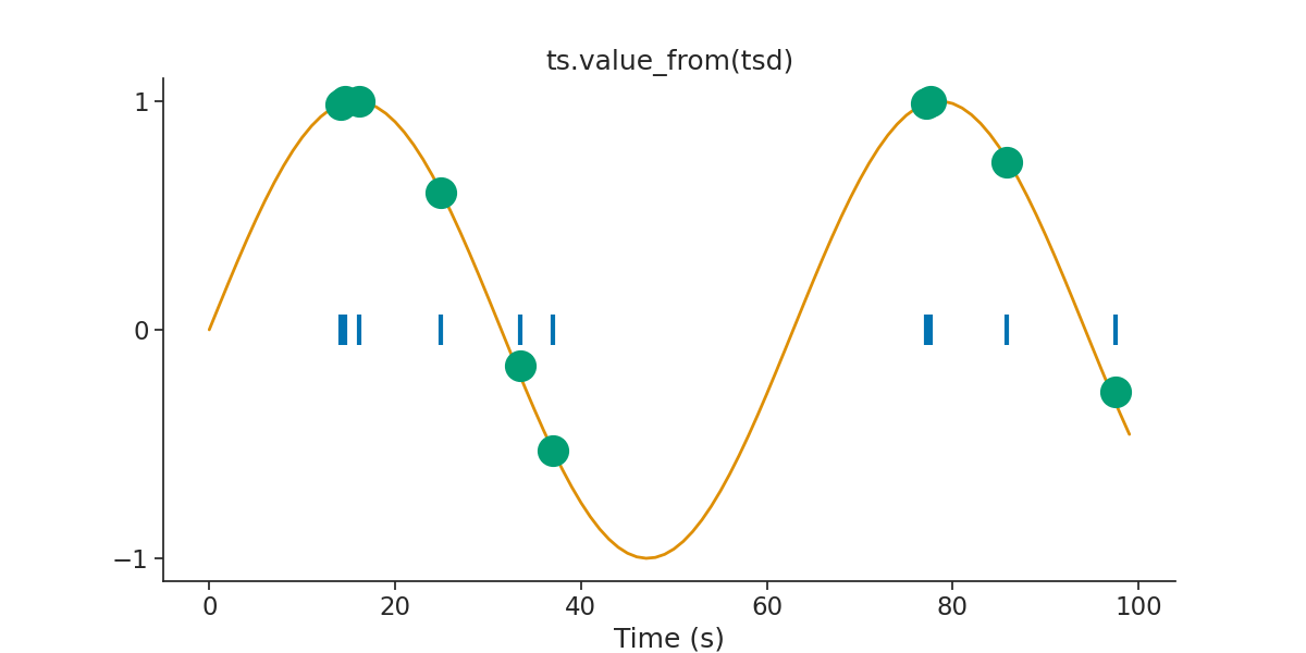
We can use value_from which as it indicates assign to every timestamps the closed value in time from another time series. Let's define the time series we want to assign values from.
tsd_sin = nap.Tsd(t=np.arange(0, 100, 1), d=np.sin(np.arange(0, 10, 0.1)))

tsgroup_sin = tsgroup.value_from(tsd_sin)

plt.figure(figsize=(12, 6))
plt.plot(tsgroup[0].fillna(0), "|", markersize=20, mew=3)
plt.plot(tsd_sin, linewidth=2)
plt.plot(tsgroup_sin[0], "o", markersize=20)
plt.title("ts.value_from(tsd)")
plt.xlabel("Time (s)")
plt.yticks([-1, 0, 1])
plt.show()
Total running time of the script: ( 0 minutes 1.784 seconds)
Download Python source code: tutorial_pynapple_core.py