Note
Click here to download the full example code
Advanced processing
The pynapple package provides a small set of high-level functions that are widely used in systems neuroscience.
- Discrete correlograms
- Tuning curves
- Decoding
- PETH
- Randomization
This notebook provides few examples with artificial data.
Warning
This tutorial uses seaborn and matplotlib for displaying the figure.
You can install both with pip install matplotlib seaborn
import numpy as np
import pandas as pd
import pynapple as nap
import matplotlib.pyplot as plt
import seaborn as sns

custom_params = {"axes.spines.right": False, "axes.spines.top": False}
sns.set_theme(style="ticks", palette="colorblind", font_scale=1.5, rc=custom_params)
Discrete correlograms
First let's generate some data. Here we have two neurons recorded together. We can group them in a TsGroup.
ts1 = nap.Ts(t=np.sort(np.random.uniform(0, 1000, 2000)), time_units="s")
ts2 = nap.Ts(t=np.sort(np.random.uniform(0, 1000, 1000)), time_units="s")
epoch = nap.IntervalSet(start=0, end=1000, time_units="s")
ts_group = nap.TsGroup({0: ts1, 1: ts2}, time_support=epoch)

print(ts_group)
Out:
First we can compute their autocorrelograms meaning the number of spikes of a neuron observed in a time windows centered around its own spikes.
For this we can use the function compute_autocorrelogram.
We need to specifiy the binsize and windowsize to bin the spike train.
autocorrs = nap.compute_autocorrelogram(
    group=ts_group, binsize=100, windowsize=1000, time_units="ms", ep=epoch  # ms
)
print(autocorrs, "\n")
Out:
           0     1
-0.9  0.9475  1.05
-0.8  0.9750  1.10
-0.7  0.9725  0.97
-0.6  1.0150  1.05
-0.5  0.9425  0.85
-0.4  0.9575  0.89
-0.3  0.9425  0.79
-0.2  1.0250  1.11
-0.1  1.0750  0.96
 0.0  0.0000  0.00
 0.1  1.0750  0.96
 0.2  1.0250  1.11
 0.3  0.9425  0.79
 0.4  0.9575  0.89
 0.5  0.9425  0.85
 0.6  1.0150  1.05
 0.7  0.9725  0.97
 0.8  0.9750  1.10
 0.9  0.9475  1.05
The variable autocorrs is a pandas DataFrame with the center of the bins for the index and each columns is a neuron.
Similarly, we can compute crosscorrelograms meaning how many spikes of neuron 1 do I observe whenever neuron 0 fires. Here the function
is called compute_crosscorrelogram and takes a TsGroup as well.
crosscorrs = nap.compute_crosscorrelogram(
    group=ts_group, binsize=100, windowsize=1000, time_units="ms"  # ms
)

print(crosscorrs, "\n")
Out:
          0
          1
-0.9  1.040
-0.8  1.110
-0.7  1.000
-0.6  1.005
-0.5  1.090
-0.4  0.875
-0.3  0.980
-0.2  1.120
-0.1  1.055
 0.0  1.045
 0.1  1.010
 0.2  1.040
 0.3  1.070
 0.4  1.045
 0.5  0.985
 0.6  0.965
 0.7  1.055
 0.8  1.170
 0.9  0.980
Column name (0, 1) is read as cross-correlogram of neuron 0 and 1 with neuron 0 being the reference time.
Peri-Event Time Histogram (PETH)
A second way to examine the relationship between spiking and an event (i.e. stimulus) is to compute a PETH. pynapple uses the function compute_perievent to center spike time around the timestamps of an event within a given window.
stim = nap.Tsd(
    t=np.sort(np.random.uniform(0, 1000, 50)), d=np.random.rand(50), time_units="s"
)

peth0 = nap.compute_perievent(ts1, stim, minmax=(-0.1, 0.2), time_unit="s")

print(peth0)
Out:
  Index       rate    ref_times
-------  ---------  -----------
      0  nan            23.9996
      1    3.33333      28.0529
      2  nan            46.6504
      3    3.33333      72.9137
      4  nan            73.5197
      5    6.66667      80.8389
      6  nan           117.547
      7  nan           141.686
      8  nan           154.962
      9  nan           160.518
     10  nan           190.095
     11    6.66667     219.417
     12    3.33333     228.274
     13  nan           241.984
     14    6.66667     264.217
     15    3.33333     299.341
     16  nan           316.922
     17  nan           331.141
     18  nan           406.893
     19  nan           422.294
     20  nan           430.157
     21    3.33333     437.542
     22    3.33333     464.405
     23  nan           482.52
     24  nan           487.688
     25    6.66667     494.404
     26  nan           507.024
     27    3.33333     531.726
     28    3.33333     556.851
     29    3.33333     559.877
     30  nan           571.838
     31  nan           647.292
     32    6.66667     709.389
     33    3.33333     809.848
     34  nan           810.405
     35    3.33333     817.995
     36  nan           866.084
     37  nan           886.307
     38  nan           894.487
     39    3.33333     896.847
     40    3.33333     897.95
     41    6.66667     928.571
     42  nan           929.996
     43  nan           933.221
     44    3.33333     933.409
     45    3.33333     938.691
     46  nan           962.453
     47    3.33333     979.04
     48    6.66667     979.768
     49    3.33333     998.711
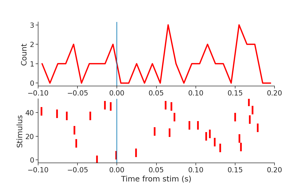
It is then easy to create a raster plot around the times of the stimulation event by calling the to_tsd function of pynapple to "flatten" the TsGroup peth0.
mkdocs_gallery_thumbnail_number = 2
plt.figure(figsize=(10, 6))
plt.subplot(211)
plt.plot(np.sum(peth0.count(0.01), 1), linewidth=3, color="red")
plt.xlim(-0.1, 0.2)
plt.ylabel("Count")
plt.axvline(0.0)
plt.subplot(212)
plt.plot(peth0.to_tsd(), "|", markersize=20, color="red", mew=4)
plt.xlabel("Time from stim (s)")
plt.ylabel("Stimulus")
plt.xlim(-0.1, 0.2)
plt.axvline(0.0)
Out:
The same function can be applied to a group of neurons. In this case, it returns a dict of TsGroup
pethall = nap.compute_perievent(ts_group, stim, minmax=(-0.1, 0.2), time_unit="s")

print(pethall[1])
Out:
  Index       rate    ref_times
-------  ---------  -----------
      0  nan            23.9996
      1  nan            28.0529
      2  nan            46.6504
      3  nan            72.9137
      4  nan            73.5197
      5  nan            80.8389
      6  nan           117.547
      7    3.33333     141.686
      8    6.66667     154.962
      9  nan           160.518
     10  nan           190.095
     11    3.33333     219.417
     12  nan           228.274
     13  nan           241.984
     14    3.33333     264.217
     15  nan           299.341
     16  nan           316.922
     17    3.33333     331.141
     18  nan           406.893
     19    3.33333     422.294
     20  nan           430.157
     21  nan           437.542
     22  nan           464.405
     23  nan           482.52
     24  nan           487.688
     25  nan           494.404
     26  nan           507.024
     27  nan           531.726
     28  nan           556.851
     29  nan           559.877
     30  nan           571.838
     31  nan           647.292
     32  nan           709.389
     33  nan           809.848
     34    3.33333     810.405
     35  nan           817.995
     36  nan           866.084
     37  nan           886.307
     38    3.33333     894.487
     39  nan           896.847
     40  nan           897.95
     41    3.33333     928.571
     42  nan           929.996
     43  nan           933.221
     44  nan           933.409
     45  nan           938.691
     46    3.33333     962.453
     47    3.33333     979.04
     48  nan           979.768
     49    3.33333     998.711
Tuning curves
pynapple can compute 1 dimension tuning curves (for example firing rate as a function of angular direction) and 2 dimension tuning curves ( for example firing rate as a function of position). In both cases, a TsGroup object can be directly passed to the function.
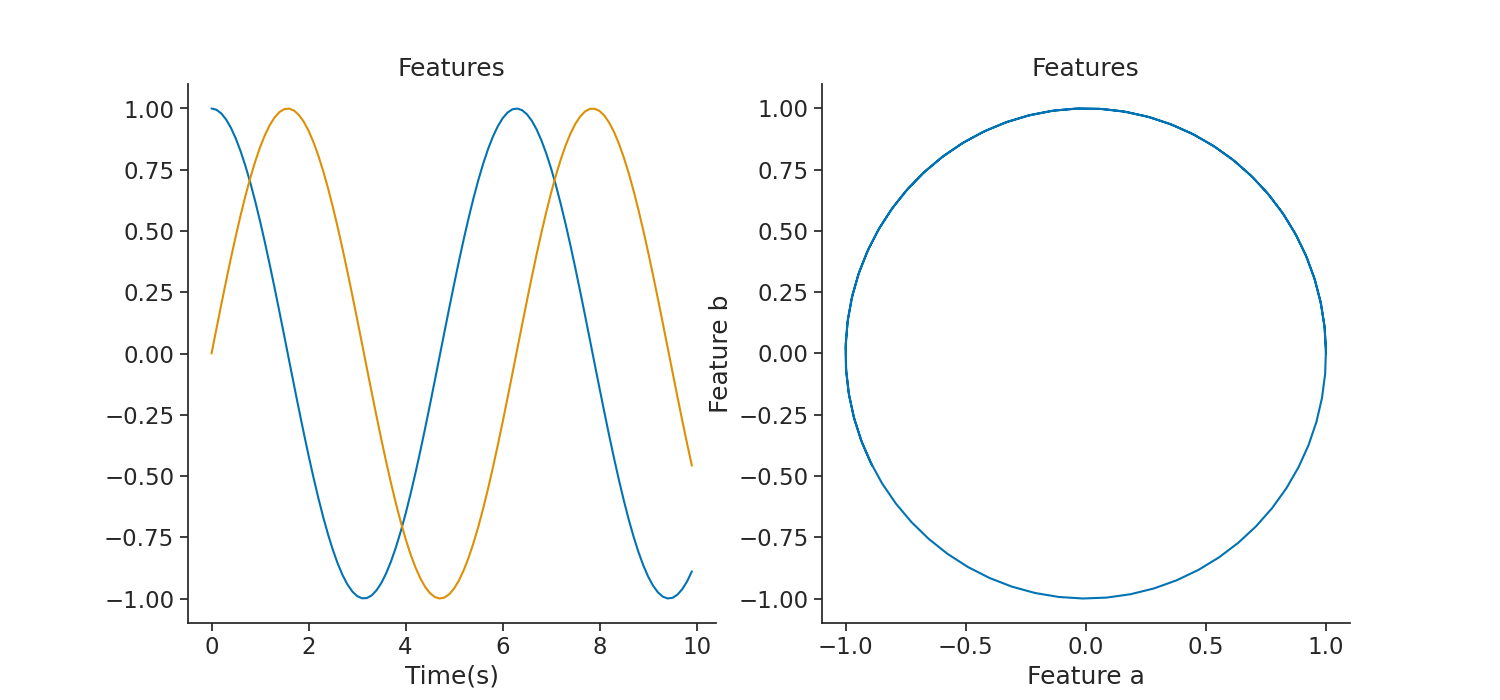
First we will create the 2D features:
dt = 0.1
features = np.vstack((np.cos(np.arange(0, 1000, dt)), np.sin(np.arange(0, 1000, dt)))).T
# features += np.random.randn(features.shape[0], features.shape[1])*0.05
features = nap.TsdFrame(
    t=np.arange(0, 1000, dt),
    d=features,
    time_units="s",
    time_support=epoch,
    columns=["a", "b"],
)

print(features)

plt.figure(figsize=(15, 7))
plt.subplot(121)
plt.plot(features[0:100])
plt.title("Features")
plt.xlabel("Time(s)")
plt.subplot(122)
plt.title("Features")
plt.plot(features["a"][0:100], features["b"][0:100])
plt.xlabel("Feature a")
plt.ylabel("Feature b")
Out:
Time (s)           a         b
----------  --------  --------
0.0          1         0
0.1          0.995     0.09983
0.2          0.98007   0.19867
0.3          0.95534   0.29552
0.4          0.92106   0.38942
0.5          0.87758   0.47943
0.6          0.82534   0.56464
0.7          0.76484   0.64422
0.8          0.69671   0.71736
0.9          0.62161   0.78333
1.0          0.5403    0.84147
1.1          0.4536    0.89121
1.2          0.36236   0.93204
1.3          0.2675    0.96356
1.4          0.16997   0.98545
1.5          0.07074   0.99749
1.6         -0.0292    0.99957
1.7         -0.12884   0.99166
1.8         -0.2272    0.97385
1.9         -0.32329   0.9463
2.0         -0.41615   0.9093
2.1         -0.50485   0.86321
2.2         -0.5885    0.8085
2.3         -0.66628   0.74571
2.4         -0.73739   0.67546
2.5         -0.80114   0.59847
2.6         -0.85689   0.5155
2.7         -0.90407   0.42738
2.8         -0.94222   0.33499
2.9         -0.97096   0.23925
...
997.0       -0.44006  -0.89797
997.1       -0.34822  -0.93741
997.2       -0.25289  -0.96749
997.3       -0.15504  -0.98791
997.4       -0.05564  -0.99845
997.5        0.04432  -0.99902
997.6        0.14383  -0.9896
997.7        0.24191  -0.9703
997.8        0.33757  -0.9413
997.9        0.42986  -0.9029
998.0        0.51785  -0.85547
998.1        0.60066  -0.7995
998.2        0.67748  -0.73554
998.3        0.74753  -0.66423
998.4        0.81011  -0.58628
998.5        0.86459  -0.50248
998.6        0.91043  -0.41365
998.7        0.94718  -0.3207
998.8        0.97447  -0.22453
998.9        0.99201  -0.12613
999.0        0.99965  -0.02646
999.1        0.9973    0.07347
999.2        0.98498   0.17267
999.3        0.96282   0.27014
999.4        0.93104   0.36491
999.5        0.88996   0.45604
999.6        0.83999   0.54261
999.7        0.78162   0.62375
999.8        0.71544   0.69867
999.9        0.64212   0.7666
dtype: float64, shape: (10000, 2)

Text(732.5909090909089, 0.5, 'Feature b')
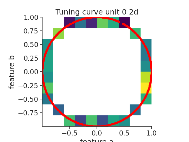
Here we call the function compute_2d_tuning_curves.
To check the accuracy of the tuning curves, we will display the spikes aligned to the features with the function value_from which assign to each spikes the corresponding feature value for neuron 0.
tcurves2d, binsxy = nap.compute_2d_tuning_curves(
    group=ts_group, features=features, nb_bins=10
)

ts_to_features = ts_group[1].value_from(features)

plt.figure()
plt.plot(ts_to_features["a"], ts_to_features["b"], "o", color="red", markersize=4)
extents = (
    np.min(features["b"]),
    np.max(features["b"]),
    np.min(features["a"]),
    np.max(features["a"]),
)
plt.imshow(tcurves2d[1].T, origin="lower", extent=extents, cmap="viridis")
plt.title("Tuning curve unit 0 2d")
plt.xlabel("feature a")
plt.ylabel("feature b")
plt.grid(False)
plt.show()
Out:
/mnt/home/gviejo/pynapple/pynapple/process/tuning_curves.py:223: RuntimeWarning: invalid value encountered in divide
  count = count / occupancy
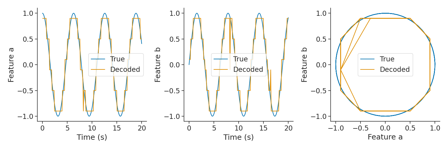
Decoding
Pynapple supports 1 dimensional and 2 dimensional bayesian decoding. The function returns the decoded feature as well as the probabilities for each timestamps.
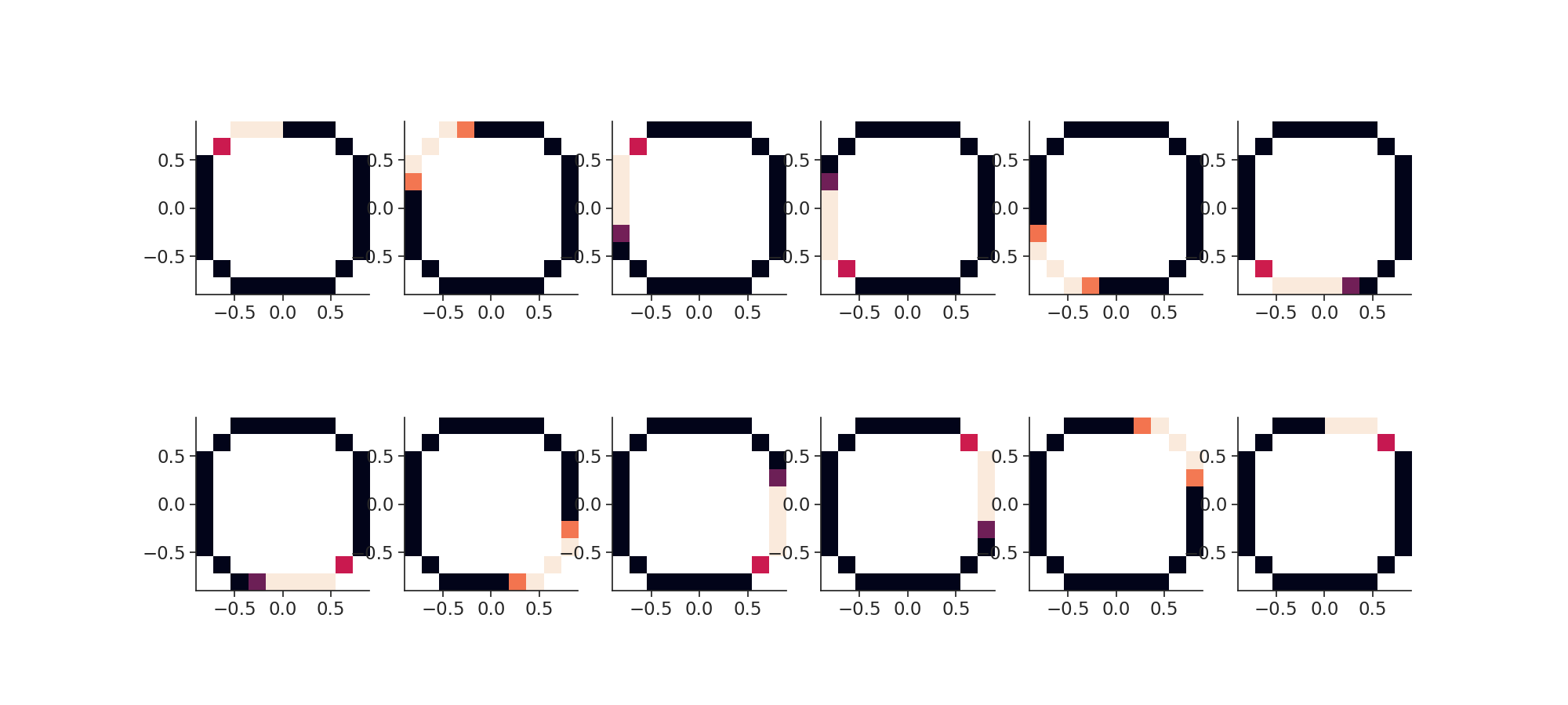
First we generate some artificial "place fields" in 2 dimensions based on the features.
This part is just to generate units with a relationship to the features (i.e. "place fields")
times = features.as_units("us").index.values
ft = features.values
alpha = np.arctan2(ft[:, 1], ft[:, 0])
bins = np.repeat(np.linspace(-np.pi, np.pi, 13)[::, np.newaxis], 2, 1)
bins += np.array([-2 * np.pi / 24, 2 * np.pi / 24])
ts_group = {}
for i in range(12):
    ts = times[(alpha >= bins[i, 0]) & (alpha <= bins[i + 1, 1])]
    ts_group[i] = nap.Ts(ts, time_units="us")

ts_group = nap.TsGroup(ts_group, time_support=epoch)
print(ts_group)
Out:
  Index    rate
-------  ------
      0   1.248
      1   1.665
      2   1.666
      3   1.664
      4   1.665
      5   1.67
      6   1.671
      7   1.673
      8   1.665
      9   1.666
     10   1.667
     11   1.248
To decode we need to compute tuning curves in 2D.
import warnings

warnings.filterwarnings("ignore")

tcurves2d, binsxy = nap.compute_2d_tuning_curves(
    group=ts_group,
    features=features,
    nb_bins=10,
    ep=epoch,
    minmax=(-1.0, 1.0, -1.0, 1.0),
)
Then we plot the "place fields".
plt.figure(figsize=(20, 9))
for i in ts_group.keys():
    plt.subplot(2, 6, i + 1)
    plt.imshow(
        tcurves2d[i], extent=(binsxy[1][0], binsxy[1][-1], binsxy[0][0], binsxy[0][-1])
    )
    plt.xticks()
plt.show()
Then we call the actual decoding function in 2d.
decoded, proba_feature = nap.decode_2d(
    tuning_curves=tcurves2d,
    group=ts_group,
    ep=epoch,
    bin_size=0.1,  # second
    xy=binsxy,
    features=features,
)


plt.figure(figsize=(15, 5))
plt.subplot(131)
plt.plot(features["a"].as_units("s").loc[0:20], label="True")
plt.plot(decoded["a"].as_units("s").loc[0:20], label="Decoded")
plt.legend()
plt.xlabel("Time (s)")
plt.ylabel("Feature a")
plt.subplot(132)
plt.plot(features["b"].as_units("s").loc[0:20], label="True")
plt.plot(decoded["b"].as_units("s").loc[0:20], label="Decoded")
plt.legend()
plt.xlabel("Time (s)")
plt.ylabel("Feature b")
plt.subplot(133)
plt.plot(
    features["a"].as_units("s").loc[0:20],
    features["b"].as_units("s").loc[0:20],
    label="True",
)
plt.plot(
    decoded["a"].as_units("s").loc[0:20],
    decoded["b"].as_units("s").loc[0:20],
    label="Decoded",
)
plt.xlabel("Feature a")
plt.ylabel("Feature b")
plt.legend()
plt.tight_layout()
plt.show()
Randomization
Pynapple provides some ready-to-use randomization methods to compute null distributions for statistical testing. Different methods preserve or destroy different features of the data, here's a brief overview.
shift_timestamps shifts all the timestamps in a Ts object by the same random amount, wrapping the end of the time support to its beginning. This randomization preserves the temporal structure in the data but destroys the temporal relationships with other quantities (e.g. behavioural data).
When applied on a TsGroup object, each series in the group is shifted independently.
ts = nap.Ts(t=np.sort(np.random.uniform(0, 100, 10)), time_units="ms")
rand_ts = nap.shift_timestamps(ts, min_shift=1, max_shift=20)
shuffle_ts_intervals computes the intervals between consecutive timestamps, permutes them, and generates a new set of timestamps with the permuted intervals.
This procedure preserve the distribution of intervals, but not their sequence.
ts = nap.Ts(t=np.sort(np.random.uniform(0, 100, 10)), time_units="s")
rand_ts = nap.shuffle_ts_intervals(ts)
jitter_timestamps shifts each timestamp in the data of an independent random amount. When applied with a small max_jitter, this procedure destroys the fine temporal structure of the data, while preserving structure on longer timescales.
ts = nap.Ts(t=np.sort(np.random.uniform(0, 100, 10)), time_units="s")
rand_ts = nap.jitter_timestamps(ts, max_jitter=1)
resample_timestamps uniformly re-draws the same number of timestamps in ts, in the same time support. This procedures preserve the total number of timestamps, but destroys any other feature of the original data.
ts = nap.Ts(t=np.sort(np.random.uniform(0, 100, 10)), time_units="s")
rand_ts = nap.resample_timestamps(ts)
Total running time of the script: ( 0 minutes 1.692 seconds)
Download Python source code: tutorial_pynapple_process.py